
Laplace Transform Table
The Laplace transform turns a function of time, f(t), into a function of a complex variable, F(s). This page lists the most common transforms and their regions of convergence, the key properties, the inverse transform with worked examples, and a finder for the standard cases. Download the table as a PDF.
Laplace Transform Finder
Pick a function f(t), set its constants, and get its Laplace transform F(s) and region of convergence.
Table of Common Laplace Transforms
Each entry gives f(t) for t ≥ 0 and its transform F(s) = ℒ{f(t)} = ∫₀^∞ e⁻ˢᵗ f(t) dt. Here a, b and c are real constants, n is a non-negative integer, u(t) is the unit step and δ(t) is the Dirac delta. The last column is the region of convergence. The exponential, sine and cosine entries use the same functions as the trigonometric table and the powers table.
Basic functions
| f(t) | F(s) = ℒ{f(t)} | Valid for |
|---|---|---|
| 1 | 1/s | Re(s) > 0 |
| t | 1/s² | Re(s) > 0 |
| tⁿ (n = 0, 1, 2, …) | n!/sⁿ⁺¹ | Re(s) > 0 |
| tᵃ (a > −1) | Γ(a + 1)/sᵃ⁺¹ | Re(s) > 0 |
| √t | √π/(2s√s) | Re(s) > 0 |
| 1/√t | √(π/s) | Re(s) > 0 |
Exponentials
| f(t) | F(s) = ℒ{f(t)} | Valid for |
|---|---|---|
| eᵃᵗ | 1/(s − a) | Re(s) > a |
| t·eᵃᵗ | 1/(s − a)² | Re(s) > a |
| tⁿ·eᵃᵗ | n!/(s − a)ⁿ⁺¹ | Re(s) > a |
Trigonometric and hyperbolic
| f(t) | F(s) = ℒ{f(t)} | Valid for |
|---|---|---|
| sin(bt) | b/(s² + b²) | Re(s) > 0 |
| cos(bt) | s/(s² + b²) | Re(s) > 0 |
| sinh(bt) | b/(s² − b²) | Re(s) > |b| |
| cosh(bt) | s/(s² − b²) | Re(s) > |b| |
| sin²(bt) | 2b²/(s(s² + 4b²)) | Re(s) > 0 |
| cos²(bt) | (s² + 2b²)/(s(s² + 4b²)) | Re(s) > 0 |
| t·sin(bt) | 2bs/(s² + b²)² | Re(s) > 0 |
| t·cos(bt) | (s² − b²)/(s² + b²)² | Re(s) > 0 |
| sin(bt)/t | arctan(b/s) | Re(s) > 0 |
Exponential times trigonometric (damped)
| f(t) | F(s) = ℒ{f(t)} | Valid for |
|---|---|---|
| eᵃᵗ·sin(bt) | b/((s − a)² + b²) | Re(s) > a |
| eᵃᵗ·cos(bt) | (s − a)/((s − a)² + b²) | Re(s) > a |
| eᵃᵗ·sinh(bt) | b/((s − a)² − b²) | Re(s) > a + |b| |
| eᵃᵗ·cosh(bt) | (s − a)/((s − a)² − b²) | Re(s) > a + |b| |
Step and impulse
| f(t) | F(s) = ℒ{f(t)} | Valid for |
|---|---|---|
| u(t − c) (c ≥ 0) | e⁻ᶜˢ/s | Re(s) > 0 |
| δ(t) | 1 | all s |
| δ(t − c) (c ≥ 0) | e⁻ᶜˢ | all s |
Properties of the Laplace Transform
These rules let you build new transforms from the table above. F(s) and G(s) are the transforms of f(t) and g(t).
| Property | Time domain | s-domain |
|---|---|---|
| Linearity | a·f(t) + b·g(t) | a·F(s) + b·G(s) |
| Frequency shift | eᵃᵗ·f(t) | F(s − a) |
| Time shift | f(t − c)·u(t − c) | e⁻ᶜˢ·F(s) |
| Scaling (c > 0) | f(ct) | (1/c)·F(s/c) |
| Multiplication by tⁿ | tⁿ·f(t) | (−1)ⁿ·dⁿF/dsⁿ |
| First derivative | f′(t) | s·F(s) − f(0) |
| Second derivative | f″(t) | s²·F(s) − s·f(0) − f′(0) |
| nth derivative | f⁽ⁿ⁾(t) | sⁿF(s) − sⁿ⁻¹f(0) − … − f⁽ⁿ⁻¹⁾(0) |
| Integration | ∫₀ᵗ f(τ) dτ | F(s)/s |
| Division by t | f(t)/t | ∫ F(σ) dσ, σ from s to ∞ |
| Convolution | (f ∗ g)(t) = ∫₀ᵗ f(τ)·g(t − τ) dτ | F(s)·G(s) |
| Periodic, period T | f(t + T) = f(t) | (1/(1 − e⁻ˢᵀ))·∫₀ᵀ e⁻ˢᵗ f(t) dt |
Initial and final value theorems
- Initial value: limt→0⁺ f(t) = lims→∞ s·F(s).
- Final value: limt→∞ f(t) = lims→0 s·F(s), valid only when every pole of s·F(s) has a negative real part.
Inverse Laplace Transform
To recover f(t) from F(s), rewrite F(s) as a sum of terms that appear in the table, then invert each term. Two techniques cover most cases:
- Partial fractions for rational functions with real poles.
- Completing the square for quadratics with complex roots, so the result matches the damped sine and cosine entries.
Example 1: real poles
Find f(t) when F(s) = (3s + 7) / ((s + 1)(s + 2)).
- Write F(s) = A/(s + 1) + B/(s + 2).
- A = (3(−1) + 7) / (−1 + 2) = 4, and B = (3(−2) + 7) / (−2 + 1) = −1.
- Invert each term with 1/(s − a) ↔ eᵃᵗ.
- f(t) = 4e⁻ᵗ − e⁻²ᵗ. Check: f(0) = 3, which equals lim s·F(s) as s → ∞.
Example 2: complex roots
Find f(t) when F(s) = (2s + 3) / (s² + 4s + 13).
- Complete the square: s² + 4s + 13 = (s + 2)² + 9.
- Split the numerator: 2s + 3 = 2(s + 2) − 1.
- F(s) = 2·(s + 2)/((s + 2)² + 9) − (1/3)·3/((s + 2)² + 9).
- Use the entries for eᵃᵗ·cos(bt) and eᵃᵗ·sin(bt) with a = −2 and b = 3.
- f(t) = e⁻²ᵗ (2cos 3t − ⅓ sin 3t).
Worked Example: Solving a Differential Equation
Solve y′ + 2y = 3 with y(0) = 1.
- Transform both sides using the derivative rule: s·Y(s) − 1 + 2·Y(s) = 3/s.
- Solve for Y(s): (s + 2)·Y(s) = 1 + 3/s = (s + 3)/s, so Y(s) = (s + 3) / (s(s + 2)).
- Partial fractions: Y(s) = (3/2)/s − (1/2)/(s + 2).
- Invert with the table: y(t) = 3/2 − ½ e⁻²ᵗ.
- Check: y(0) = 1, and y′ + 2y = e⁻²ᵗ + 3 − e⁻²ᵗ = 3.
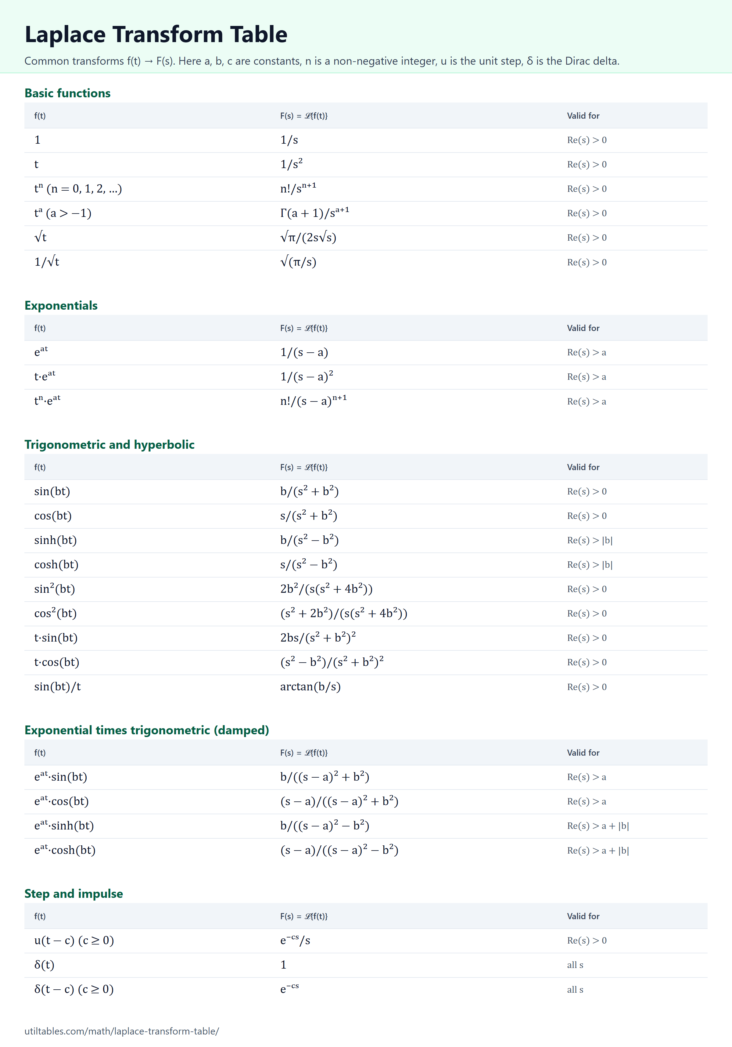
Laplace Transform Table as an Image and PDF
Save or print the table of common transforms. Download the PDF (it also includes the properties and the value theorems).
Frequently Asked Questions
What is the Laplace transform used for?
It converts differential equations into algebraic equations in s, which are easier to solve. It is widely used for circuits, control systems and mechanical vibrations, and it builds initial conditions directly into the solution.
When does the Laplace transform exist?
For a function that is piecewise continuous and of exponential order, the integral converges for all s with a large enough real part. That set of values of s is the region of convergence listed in the last column of the table.
What does Re(s) > a mean?
It means the real part of s must be greater than a for the integral to converge. For example, the transform 1/(s − 2) of e²ᵗ is valid only when Re(s) > 2.
How is the Laplace transform related to the Fourier transform?
When the imaginary axis lies inside the region of convergence, the Fourier transform equals the Laplace transform evaluated at s = iω. The Laplace transform also handles functions that grow exponentially, which the Fourier transform usually cannot.